[Python] 정규분포와 파레토 분포 구현

예제1

[In]

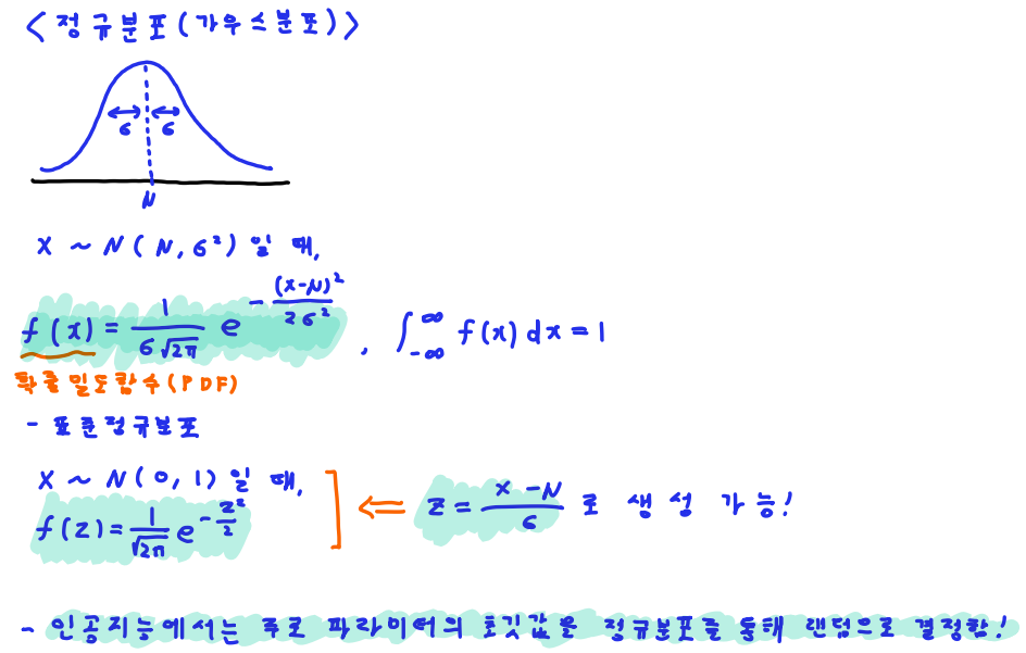
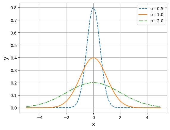
# 정규분포
%matplotlib inline

import numpy as np
import matplotlib.pyplot as plt

# 정규분포 확률밀도함수
def pdf(x, mu, sigma):
    return 1/(sigma*np.sqrt(2*np.pi))*np.exp(-(x-mu)**2/(2*sigma**2))

x = np.linspace(-5, 5, 1000)
y_1 = pdf(x, 0.0, 0.5) # 평균 : 0, 표준편차 : 0.5
y_2 = pdf(x, 0.0, 1.0) # 평균 : 0, 표준편차 : 1.0
y_3 = pdf(x, 0.0, 2.0) # 평균 : 0, 표준편차 : 2.0

plt.plot(x, y_1, label = 'σ : 0.5', linestyle = 'dashed')
plt.plot(x, y_2, label = 'σ : 1.0', linestyle = 'solid')
plt.plot(x, y_3, label = 'σ : 2.0', linestyle = 'dashdot')
plt.legend()

plt.xlabel('x', size = 14)
plt.ylabel('y', size = 14)
plt.grid()

plt.show()

[Out]

 

예제2

[In]

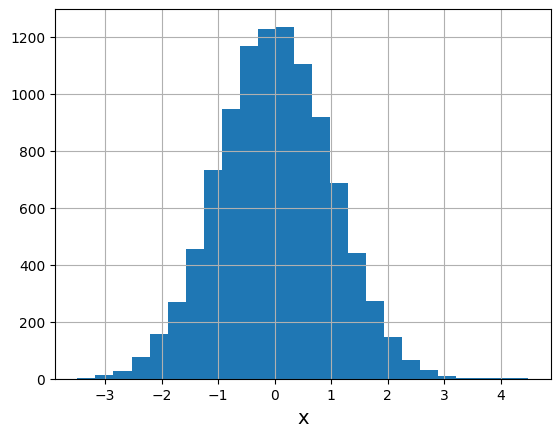
# 정규분포를 따르는 난수
%matplotlib inline

import numpy as np
import matplotlib.pyplot as plt

# 정규분포를 따르는 난수 생성
s = np.random.normal(0, 1, 10000) # 평균 : 0, 표준편차 : 1, 10000개 -> 표준정규분포

# 히스토그램
plt.hist(s, bins = 25) # bins는 기둥의 수

plt.xlabel('x', size = 14)
plt.grid()

plt.show()

[Out]

 

[In]

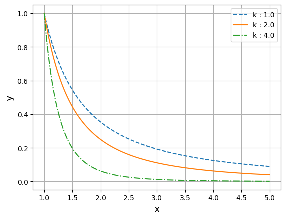
# 거듭제곱 법칙
%matplotlib inline

import numpy as np
import matplotlib.pyplot as plt

# 거듭제곱 법칙 함수
def power_func(x, c, k):
    return c*x**(-k)

x = np.linspace(1, 5, 1000)
y_1 = power_func(x, 1.0, 1.5) # c : 1.0, k : 1.5 
y_2 = power_func(x, 1.0, 2.0) # c : 1.0, k : 2.0
y_3 = power_func(x, 1.0, 4.0) # c : 1.0, k : 4.0

plt.plot(x, y_1, label='k : 1.0', linestyle = 'dashed')
plt.plot(x, y_2, label='k : 2.0', linestyle = 'solid')
plt.plot(x, y_3, label='k : 4.0', linestyle = 'dashdot')
plt.legend()

plt.xlabel('x', size = 14)
plt.ylabel('y', size = 14)
plt.grid()

plt.show()

[Out]

 

 

예제1

[In]

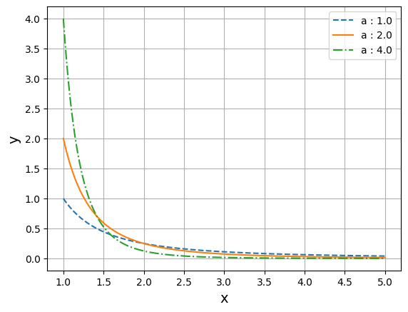
# 파레토 분포

%matplotlib inline

import numpy as np
import matplotlib.pyplot as plt

def pareto_func(x, a, m):
    return a * (m**a / x**(a + 1))

x = np.linspace(1, 5, 1000)
y_1 = pareto_func(x, 1.0, 1.0) # a : 1.0, m : 1.0
y_2 = pareto_func(x, 2.0, 1.0) # a : 2.0, m : 1.0
y_3 = pareto_func(x, 4.0, 1.0) # a : 4.0, m : 1.0

plt.plot(x, y_1, label='a : 1.0', linestyle = 'dashed')
plt.plot(x, y_2, label='a : 2.0', linestyle = 'solid')
plt.plot(x, y_3, label='a : 4.0', linestyle = 'dashdot')
plt.legend()

plt.xlabel('x', size = 14)
plt.ylabel('y', size = 14)
plt.grid()

plt.show()

[Out]

 

예제2

[In]

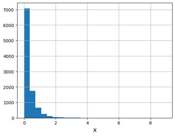
# 파렌토 분포를 따르는 난수
%matplotlib inline

import numpy as np
import matplotlib.pyplot as plt

# 파레토 분포를 따르는 난수 생성
s = np.random.pareto(4, 10000) # a : 4.0, m : 1.0, 10000개

# 히스토그램
plt.hist(s, bins = 25)
plt.xlabel('x', size = 14)
plt.grid()

plt.show()

[Out]